How To Remove Minus Sign From Percentage In Excel
Right-click one of the selected cells then click the Format Cells option. Because of the way Excel handles percentages it sees these formulas as exactly the same thing.

How To Remove Leading Minus Sign From Numbers In Excel
The Formula number1-percentage_decrease How does the formula work.

How to remove minus sign from percentage in excel. Highlight cells to remove from Use Findreplace from top Home menu Find replace - will convert to 100x. In the example shown the formula in cell E5 is. Select the columnRow that your X axis numbers are coming from.
Click Home Find Select Replace see screenshot. This negative number is enclosed in parenthesis and also displayed in blue. IF A1-B1 A1005out of limits IF B1-A1 A1005out of limits within limits This works fine but the formula is a.
Type the first number followed by the minus sign followed by the second number. Select the cell s containing the percentage symbol s that you want to remove. In the Find and Replace dialog under the Replace tab type the negative sign.
This will result in the same values in both cases because 15 015. Decrease number by percentage then use this formula. Select the range that you want to remove the negative sign.
Where 281-29281 should then equal 90 Total hours present minus total hours absent divided by total hours present. To do this modify the formula shown above by replacing the multiplication sign with a plus sign. Select the numbers and then right click to shown the context menu and select Format Cells.
The new result is multiplied by the price to get the price after the discount. From the list of options under Category select Custom Right now the format is 000. To explain how it works the semi colon divides the format between.
To decrease a number by a specific percentage you can use a formula that multiplies the number by 1 minus the percentage. Number 1 - For example heres how. If you wish to subtract percentage from a number ie.
This is the default Excel formatting. Complete the formula by pressing the Enter key. In the Type box enter the code below.
How to remove leading minus sign from numbers in Excel. Number 1 is subtracted by the percentage discount. 0000 Description of putting a plus in front of a percentage difference eg.
An alternative but more long-winded calculation would be to calculate 10 of the number and then subtract it from the original number with one of these formulas. I then went to FORMAT CELLS and clicked on PERCENT to convert the answer to a percentage. Custom Number Formatting in Excel can be used to hide percentage sign without changing the values.
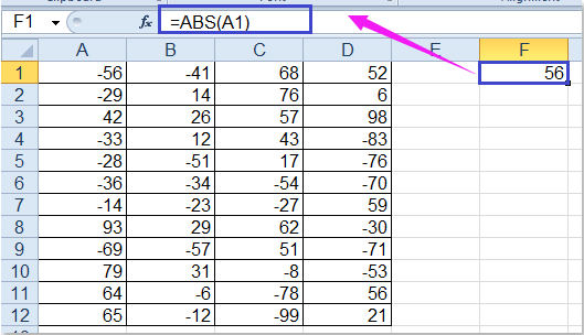
Raw data for excel practice download. We now have the number without the negative sign. Thats a quick fix.
Select Format Cells Select Number Under the box that has variations of negative numbers select the one that is red without the negative sign. How to subtract percentages. Remove negative sign from numbers with Find and Replace command.
Excel will show you the code it uses to create the percentage format you should see 000 As shown in the image below you can change this by typing in the Type section. Now immediately click on the Custom option. Blue 0 Each symbol has a meaning and in this format the represents the display of a significant digit and the 0 is the display of an insignificant digit.
Inserting -1 into the formula multiplies the number by negative 1 therefore placing the negative sign in front of it. C5 1 - D5 The results in column E are decimal values with the percentage number format applied. If there is some other way.
Select the cells containing numbers and press Ctrl 1 to activate the Format Cells dialog. In the Format Cells dialog under Number tab select Number from the Category list and the go to the right section and type 0. For example to subtract a few numbers from 100 type all those numbers separated by a minus sign.
Putting this together with the LEFT function and adding minus 1 to the formula pulls only 5 of the first 6 characters of the cell leaving the negative sign behind. To find out the price after the discount the discount percentage must be deducted by number 1. Select cells from C2 to C3 navigate to Home Number and change Percentage to General.
Select the type of formatting that you would rather use then click the OK button. BS6-BT6BS6 to get percent of time attended. 10 0010 Change the number format to include the plus or - minus sig.
Like in math you can perform more than one arithmetic operation within a single formula. But I have to write it. B21-C2 First Excel will calculate the formula 1-C2.

Salary Sheet Limited Company For Microsoft Excel Advance Formula Youtube Microsoft Excel Excel Salary

How To Change The Pivot Table Style In Excel Tutorial Excel Tutorials Pivot Table Microsoft Excel Tutorial

How To Mark Or Highlight Unique Or Duplicate Values In Excel Excel Tutorials Excel Tutorial

How To Remove Leading Minus Sign From Numbers In Excel

How To Remove Negative Sign From Numbers In Excel

How To Display Negative Percentages In Red Within Brackets In Excel Excel Tutorials Excel Negativity

How To Remove Negative Sign From Numbers In Excel

How To Create Hyperlinked Index Of Sheets In Excel Workbook Workbook Excel Tutorials Excel

How To Remove Negative Sign From Numbers In Excel


How To Remove Negative Sign From Numbers In Excel
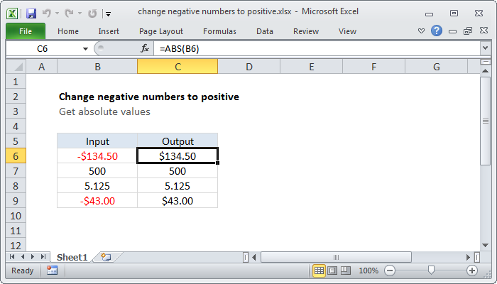
Excel Formula Change Negative Numbers To Positive Exceljet

Vlookup Formula To Compare Two Columns In Different Sheets Column Compare Formula

How To Mark Negative Percentage In Red In Microsoft Excel Excel Tutorials Microsoft Excel Excel
How To Remove Negative Sign From Numbers In Excel

How To Remove Leading Minus Sign From Numbers In Excel

How To Use Grade Formula In Excel In Urdu Hindi Excel Being Used Grade
How To Remove Negative Sign From Numbers In Excel

How To Remove Leading Minus Sign From Numbers In Excel