How To Make Negative Numbers Red And Parentheses In Excel

24 Jul, 2021

Then go to Custom and adapt to change negative to red. In accounting and financial models sometimes you will want to show negative numbers in brackets and in red color.

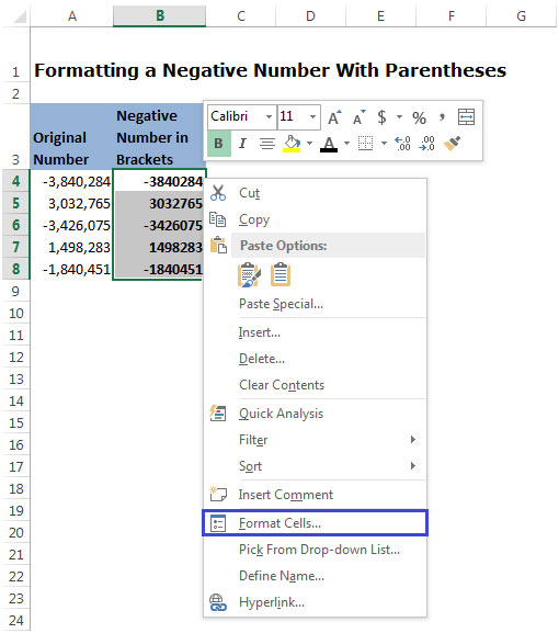
Formatting A Negative Number With Parentheses In Microsoft Excel

Right click on the cell that you want to format.

How to make negative numbers red and parentheses in excel. On Format Cells under Number tab click Custom then under Type enter 0Red-0. Motor vehicle maintenance. On the Numbers tab for Negative number format choose 11 On the Currency tab for Negative currency format choose 11 Click OK and then click OK again.

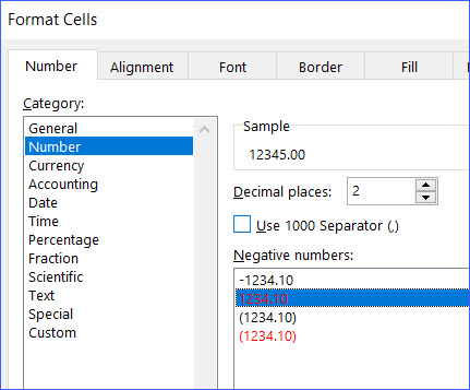
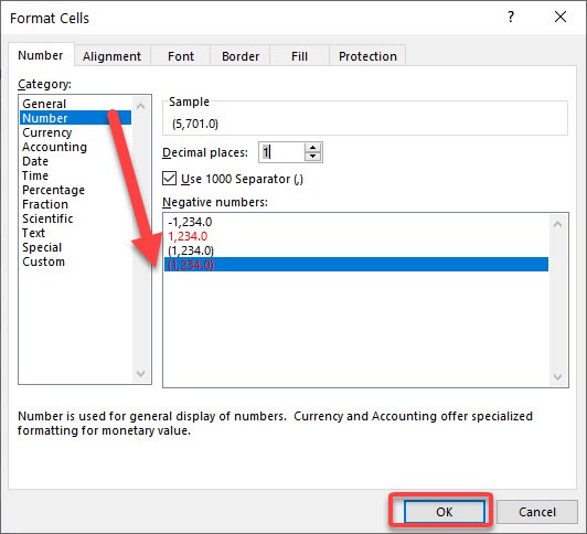
Select the Number tab and from Category select Number. This is what we would have to enter in the Type box. In the Negative Numbers box select the last option as highlighted.

One thing to note here is that Excel will display different built-in options depending on the region and language settings in your operating system. In black with a preceding minus sign. Then the numbers line up nicely.

Select the list contains negative numbers then right click to load menu. Red 0. You can also change the font color to red.

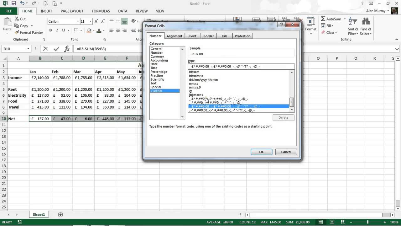
Make All Negative Numbers Red by Format Cells Setting. The _ and _ just reserve room for the and. Click on Format Cells orPress Ctrl1 on the keyboard to open the Format Cells dialog box.

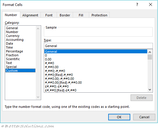
These are samples that Excel presents to us to give us an idea but we can create our own format. Use this maintenance schedule template to define the cleaning and organizing tasks to be done around the office. Verify that after above setting all negative numbers are marked in red.

Select the cells right click on the mouse. Click Format Cells on menu. Mark negative percentage in red by creating a custom format.

For example if we want to display a negative number format in red between parentheses and without decimals the format to create would be the following. When a formula returns a negative percentage the result is formatted as -49. Right click the selected cells and select Format Cells in the right-clicking menu.

Decimal places and currency. You can create a custom format to quickly format all negative percentage in red in Excel. In this video I will show you how to show negative numbers in red color andor with bracketsThis can be done using two methods-- Conditional Formatting--.

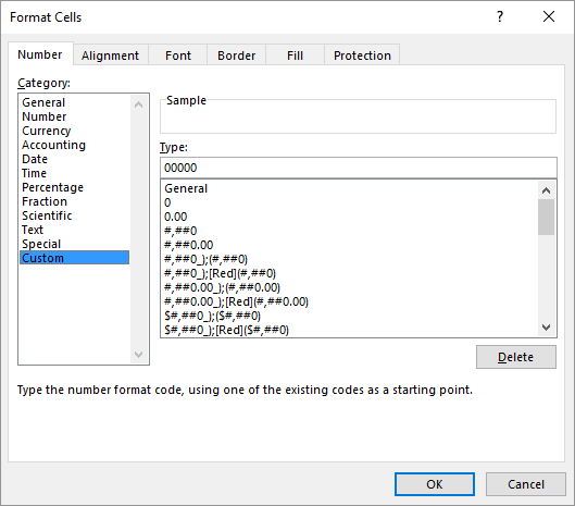
Open the dialog box Format Cells using the shortcut Ctrl 1 or by clicking on the last option of the Number Format dropdown list. Now we want to make all negative numbers in red. Positivenegative0text is the order of that formatting string.

Select the cells which have the negative percentage you want to mark in red. Click on Format Cells. Go to format cells choose the desired accounting format ie.

Manually editing excel worksheet need my edits to save as written incsv without reformatting back. If youre using Windows press Ctrl1. To display your negative numbers with parentheses we must create our own number format.

Use the following Custom Format Code to display negative numbers in red with a pair parentheses around them 000Red000 All those negative numbers in. To so so follow the following steps. Highlight the range that you want to change then right-click and choose Paste Special from the context menu to open the Paste Special dialog box.

Then click OK to confirm update. You can select the number with a minus sign in red in parentheses or in parentheses in red. Or by clicking on this icon in the ribbon Code to customize numbers in Excel.

That produces the Format Cells screen see right. Tap number -1 in a blank cell and copy it. From the Number sub menu select Custom.

Red tells excel to make the negative numbers red and the make sure that negative number is in parentheses. To Format the Negative Numbers in Red Color with brackets. We have some negative numbers in column B.

With the target cell s highlighted click on Format Cells or right-click Format Cells. How to display negative numbers in brackets in excel. You can display negative numbers by using the minus sign parentheses or by applying a red color with or without parentheses.

In this Advanced Excel tutorial you are going to learn ways. If youre using a Mac press 1. Is there any format in Excel 2002 that allows for it to be formatted 49--Dave Peterson.

Enter 0 in the Decimal. For example you may want to show an expense of 5000 as 5000 or -5000. For those in the US Excel provides the following built-in options for displaying negative numbers.

In parentheses you can choose red or black. Select the cell or range of cells that you want to format with a negative number style.

Formatting A Negative Number With Parentheses In Microsoft Excel