How To Show Negative Percentage In Excel Pie Chart
If you create a pie chart Excel charts negative values as if they were positive in other words it uses the absolute value. Click on the button on the top right of the chart and check the Data Labels checkbox.

Best Excel Tutorial Pie Of Pie Chart
The values you have used for your pie chart cause what you are percieving as a problem.

How to show negative percentage in excel pie chart. If by some reason you really have to show negative values in a pie chart which in our project we do you may consider using the following style. For instance six slices that make up 10 of the total. Pie charts arent designed to display negatives.
22122 018033 18. Click on the sign that appears on the top right of the chart and click on the arrow next to Data Labels. Add major horizontal gridlines and set color of gridlines to very light gray.
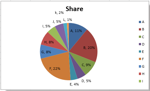
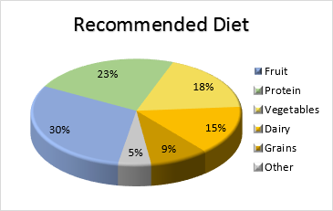
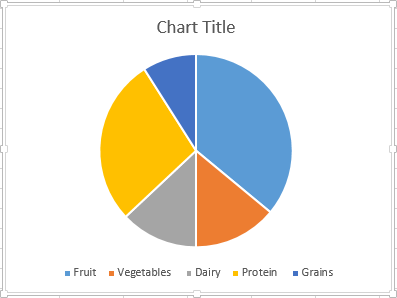
Pie charts are great but they are difficult to visualize when they have many small slices. But that doesnt reflect the percentage values bottom chart to the right. Navigate to Insert Charts Pie Chart.
Click on the chart. Go to the menu Chart tool Format select Label format and Custom. The second method is shown below.
100122 0819672 82. Choose the way you want the pie chart to be displayed. Select the data click Insert tab chose pie chart ribbon Pie of pie chart as shown below Pie of Pie chart in Excel Step 2.
The bottom chart to the right is maybe misleading but it is correct in the sense that all values are represented correctly compared to each other. You can try an expression like. Pie of Pie chart in Excel Step 1.
If SUM YourValue0SUM YourValue this will show only positive value. Show percentage in pie chart in Excel. You are using the values 100 and 22 as the slices for the pie.
You may however prefer to have the negative values charted as if they were zeroto not have a slice of the pie. You can do if SUM YourValue. The total is 122 100 22 and the percentage for each value of the total is.
Add chart title type a title text you like and decrease font size a little. 3 As a result you wont see the 0 values in your chart. Otherwise it assigns solid colors based on which point it is.
Then a pie chart is created. Fabs SUM YourValue fabs make values absolute. 2 Go to the section Number and add a new Format Code.
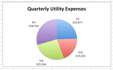
Here is the current chart we are almost done. Right click the pie chart and select Add Data Labels from the context menu. In the above chart the summation of all values is 19000 and pie area only illustrate the comparison of the absolute values for each component.
Now the corresponding. Excel outputs the absolute value of all values. To add data labels using this technique you should just right click on the chart and select the Add Data Labels option.
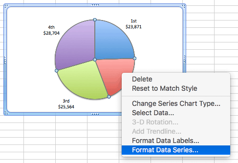
Click Kutools Charts Positive Negative Bar Chart. From the list of options some of them will display percentages. On the Format tab in the Current Selection group click the arrow next to the Chart Elements box and then click a data series.
It only addresses a chart with two data points. If you want to show values whenever they positive or negative you can use. With the Positive Negative Bar Chart tool of Kutools for Excel which only needs 3 steps to deal with this job in Excel.
If the value of a point is less than zero it colors it with a red hashed fill. In the popping dialog choose one chart type you need the choose the axis labels two series values separately. If I just leave the negative item out of the data range the remaining pie pieces are off because the negative item affects the summation value that is used to calculate the percentages.
Under Doughnut Hole Size drag the slider to the size that you want or type a percentage value between 10 and 90 in the Percentage box. Excels pie charting treats the number as as it it was a positive number and makes it part of the chart. Normally people create pie charts based on a simple set of values.
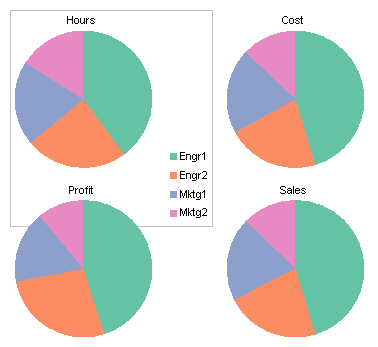
The two top charts show equal sizes for the segments in the pie thats because the relative sizes are shown. The only way to tell the number is negative is to reference the legend. Go to Chart Tools Design Chart Layouts Quick Layout.
The first method is the easiest. Select the data you will create a pie chart based on click Insert I nsert Pie or Doughnut Chart Pie. On the Format tab in the Current Selection group click Format Selection.
Percentage Pie Chart - Negative Values Reprentation This code is limited in scope. Change fill color for Negative Diff. So -20 is output in the pie chart as a slice with 20 of the pies circumference.

How To Create A Pie Chart In Excel Smartsheet

How To Make A Pie Chart In Excel
How To Display Leader Lines In Pie Chart In Excel

How To Make A Pie Chart In Excel
How To Make A Dynamic Excel Pie Chart With 4 Steps In Less Than 4 Minutes Excel Dashboard Templates
Automatically Group Smaller Slices In Pie Charts To One Big Slice


How To Show Negative Values In A Pie Chart User Experience Stack Exchange
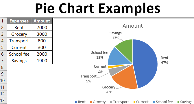
Pie Chart Examples Types Of Pie Charts In Excel With Examples
How To Create A Pie Chart In Excel Smartsheet
How To Make A Pie Chart In Excel

Creating Pie Of Pie And Bar Of Pie Charts Pie Chart Examples Pie Chart Chart
Column Chart To Replace Multiple Pie Charts Peltier Tech
Negative Values In Pie Charts Stack Overflow
How To Create A Pie Chart In Excel Smartsheet

How To Make A Pie Chart In Excel
Negative Value In Pie Chart
How To Create A Pie Chart In Excel Smartsheet
How To Make A Pie Chart In Excel

Pie Chart Mathcaptain With Pie Graph Example22376 Pie Chart Template Pie Chart Pie Graph